See also SliceTimingRikEmail
The problem
The “slice-timing” problem refers to the fact that, with a continuous descending EPI sequence for example, the bottom slice is acquired TA~=TR seconds later than the top slice. If a single basis function (such as a canonical HRF) were used to model the response, and onset times were specified relative to the start of each scan, the data in the bottom slice would be delayed by TR seconds relative to the model. This would produce poor (and biased) parameter estimates for later slices, and mean that different sensitivities would apply to different slices. One solution to this problem is to interpolate the data during preprocessing as if the slices were acquired simultaneously. This works reasonably well for TRs around 3 seconds (see http://www.mrc-cbu.cam.ac.uk/~rh01/henson-1999-hbm-slice.pdf).
However, a problem with slice-timing correction is that the interpolation will alias frequencies above the Nyquist limit 1/(2TR). Ironically, this means that the interpolation accuracy decreases as the slice-timing problem (ie TR) increases. For longer TRs, the severity of the interpolation error may depend on whether appreciable signal power exists above the Nyquist limit (which is more likely for rapid, randomised event-related designs). Rapid, uncorrected movements will also cause errors in the interpolation, even for short TRs. For these reasons, some people prefer an alternative solution to the slice-timing problem, which is keep the data unchanged, but have a more complex model, ie to accommodate the timing errors within the GLM. One can add the temporal derivatives of one's temporal basis functions for example, to "mop up" latency differences between slices (see http://www.mrc-cbu.cam.ac.uk/~rh01/henson-1999-hbm-slice.pdf). SPM's temporal derivative of its canonical HRF can handle latency differences of approx +/-1s for example, making it sufficient for TRs of up to 2s, if the model is synchronised with the middle slice (and if all brain regions exhibited a canonical response). If one suspects additional latency differences owing to variations in the vasculature of different brain regions, then even more basis functions may be required.
Note that if you choose to add a further regressor representing temporal derivative of an assumed HRF, this will reduce the residual error and hence improve statistics for 1st-level analyses, but will not necessarily affect 2nd-level analyses on the assumed HRF alone (since basis functions are normally orthogonal to one another, in which case the parameter estimate for the assumed HRF is unchanged by the additional of its derivative). Instead, one can include (contrasts of) the parameter estimates for the temporal derivative in 2nd-level analyses as well, and make inferences using F-contrasts (or one can combine the parameter estimates to get a "latency-independent" amplitude estimate, accurate up to the time-shift of the derivative http://www.ncbi.nlm.nih.gov/entrez/query.fcgi?db=pubmed&cmd=Retrieve&dopt=AbstractPlus&list_uids=15110015&query_hl=1&itool=pubmed_docsum). Finally, note that in some designs with very short, fixed SOAs (<~2s), the use of a temporal derivative may not be advisable, because its associated regressor will become highly correlated with the differences between different event-types (ie one will be unable to distinguish latency differences from amplitude differences).
Order of slice timing and motion correction
Slice timing correction involves resampling through time but not moving images, while motion correction involves moving images relative to each other. There is no simple answer to which should be done first. If slice timing is done first, then if there are abrupt movements between scans, the interpolation across time will be blurring across voxels from different parts of the brain in its correction. If motion correction is done first, then the slices in the image no longer always correspond to order of acquisition of the slices, and the temporal correction applied won't be appropriate.
If you use an interleaved slice order during acqusition (no longer the default at the CBU - see discussion of slice order then you will probably want to apply slice timing before motion correction. Because all of the odd-numbered slices are acquired first, and the all the even ones, adjacent slices are acquired apart in time (0.5 * TR = around a second). A shift in the image by motion correction of 1 slice (4 mm) will cause a substantial shift in acqusition time for a particular slice, and slice timing will not be at all appropriately applied.
A disadvantage of doing motion correction before slice timing is that an extra reslicing stage is required in between (i.e., you must generate r* images before doing slice timing).
If you use a sequential slice order during acquisition, many people prefer to apply motion correction before slice timing. I do not know if this has been evaluated in any thorough way.
Interpolation and slice timing
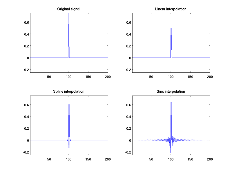
Slice timing involves interpolation in time. There are a variety of methods of interpolation - linear merely takes the values either side of the required new value, and takes a weighted average of the two, using weights inversely proportional to the distance of the new point from the original values. More complicated schemes (using more distant data points) include spline and sinc interpolation. Methods using more data points will tend to spread local artefacts across a larger part of the time series. For example, here are the effects of different methods of interpolation on a time series containing a single spike:

Note that SPM uses sinc interpolation for slice timing, so will tend to spread artefacts over a wide time window. (MatthewBrett)