Contents
Introduction
The presence of physiological noise in functional MRI can greatly limit the sensitivity and accuracy of BOLD signal measurements, and produce significant false positives. There are two main types of physiological confounds: (1) high-variance signal in non-neuronal tissues of the brain including vascular tracts, sinuses and ventricles, and (2) physiological noise components which extend into gray matter tissue. These physiological effects may also be partially coupled with stimuli (and thus the BOLD response).
One of the major challenges of BOLD fMRI is to identify and control BOLD physiological signal. These confounds are caused by a variety of mechanisms, including
- the flow of blood and cerebrospinal fluid (CSF) driven by cardiac pulsation (Dagli et al., 1999);
- phase distortion and motion artifact due to respiration (Raj et al., 2001; Windischberger et al., 2002);
- fluctuations in O2/CO2 levels, driven by changes in respiratory and cardiac rates (Wise et al., 2004; Birn et al., 2006; Shmueli et al., 2007);
- less studied phenomena, such as vasomotion (Mayhew et al., 1996) and metabolic-linked (Yang et al., 2009) effects.
The changes in fMRI signal due to physiological effects have complex, subjectdependent spatial and temporal structure, making them difficult to separate from the BOLD response.
(The above is taken from: Churchill, N. W., & Strother, S. C. (2013). PHYCAA+: An Optimized, Adaptive Procedure for Measuring and Controlling Physiological Noise in BOLD fMRI. Neuroimage. http://www.ncbi.nlm.nih.gov/pubmed/23727534.)
One possible approach to this problem - measure respiratory and cardiac data during scanning and use it as a nuisance regressor in GLM. This page will cover two main topics:
- How to do this at the CBU?
- Is it worth doing?
Physiological noise measurement at the CBU MRI facility
At the CBU MRI facility we have two bits of equipments for this purpose:
- Pulse oxiometer (cardiac data)
- Pneumatic breathing belt (respiratory data)
The general workflow is as follows:
- Radiographers attach the equipment to participant's body at the beginning of the scanning session
- Log files are written onto the scanner's computer. The logging needs to be started manually by the radiographers and it's useful to remind them of that.
- Radiographers copy the files to network space. Again, this has to be done manually by the radiographers, who will also tell you where exactly in the network space your files are located.
- You need to extract run-specific data from the log files, since the log is continuous and starts before scanning and ends some time after the scanning has stopped.
- From the run-specific log data you need to estimate the signal phases so that can be used as a covariate in GLM
The next section will describe the last three points in detail.
Working with log files
First, you need to copy subject's log files from the network to somewhere you can process them with Matlab (presumaly your home or imaging space). For each subject two files are relevant:
- Pulse data: .PULS file, as in SUBJECTCODE_STUDYCODE.PULS
- Respiratory data: .RESP file, as in SUBJECTCODE_STUDYCODE.RESP
There are two more files (.ECG and .MAT) but currently neither contain relevant data.
Next, data relevant to the scanning runs needs to be extarcted from the log files. This is not trivial since physiological recording starts before scanning (as the equipment is attached to the participant's body) and continues without pause until the scanning is over (plus some time it takes the radiographers to detach the equipment). As a result direct syncing between scans and physiological data is not possible. The pulse data files have two timestamps - one from the PMU, and one from the MCPU, which is the same clock also used to timestamp the dicom files. I have written a matlab function which extracts relevant data based on dicom headers. It takes four inputs:
- Logfile (.PULS or .RESP file) full path
- Dicom folder full path
- TR used in the scanning run (seconds)
- Hz - frequency at which log files were recorded (at CBU this is by default 50, though the script will estimate and display this frequency from data alone as well).
The code can be downloaded from here and should be quite self-explanatory -- any questions send me an email: kristjan.kalm@mrc-cbu.cam.ac.uk
You can also use Exvolt
(https://cfn.upenn.edu/aguirre/wiki/public:pulse-oximetry_during_fmri_scanning#exvolt), though it's written in C and I wasn't able to compile this successfully on CBU machines without admin rights.
Estimating signal phases for GLM
There are couple of toolboxes written to aid with noise modelling, e.g.:
Check also:
A guide from Geoff Aguirre
(https://cfn.upenn.edu/aguirre/wiki/public:pulse-oximetry_during_fmri_scanning)Chris Rorden's Neuropsychology Lab website
(http://www.mccauslandcenter.sc.edu/CRNL/tools/part)
In the analysis below I have used PhleM since it's written in MATLAB.
Is it worth it - a quick evaluation of the effect of noise regressors
Here I have used 2 datasets: (1) visually presented houses vs faces, (2) retinotopic mapping task.
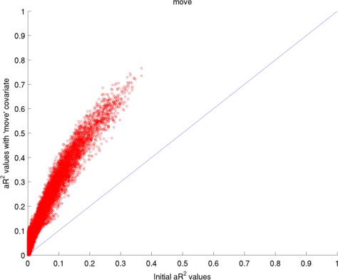
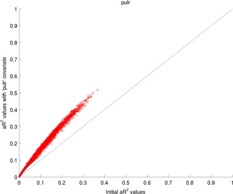
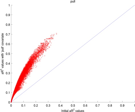
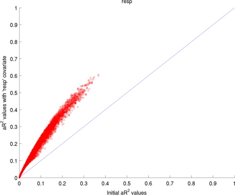
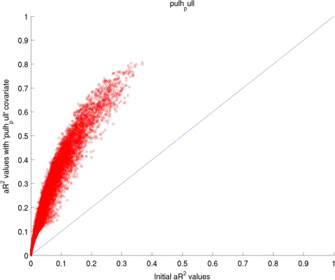
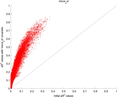
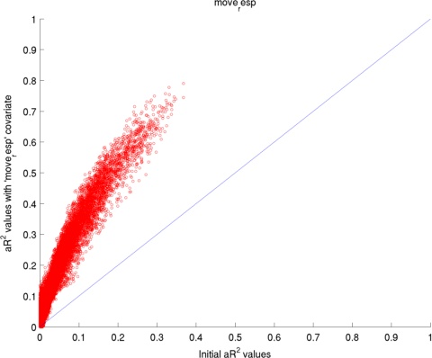
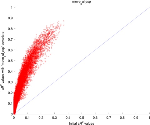
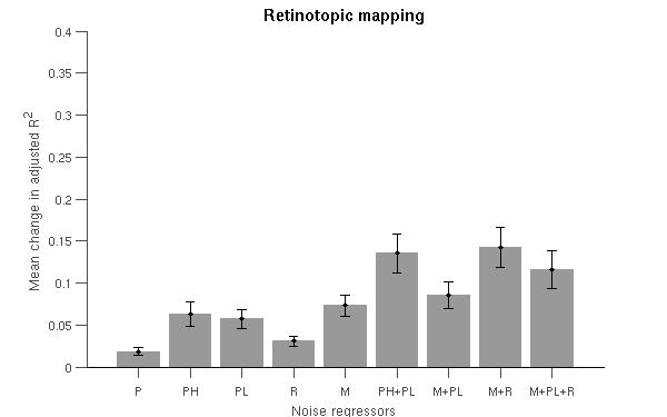
The figures below present the average change in adjusted coefficient of determination (R2) values for the voxels in the occipital and inferior temporal lobe. The adjusted coefficient of determination (aR2) was calculated at each voxel to compare the proportion of time series variance accounted for by each of the models while adjusting for the different numbers of regressors in each of the models. aR2 is defined as aR2 = 1 - (SS_err / SS_tot) (df_tot / df_err), where SS_err = (standard deviation of the residual errors)2, SS_tot = (standard deviation of time series)2, df_tot = number of degrees of freedom in the data - 1, and df_err = df_tot - 1 — number of degrees of freedom in each model. The resulting aR2 values were averaged over voxels within the reqion of interest and then over subjects.
The ROI for 'Houses vs. Faces' is the inferior temporal lobe and the ROI for 'Retinotopic mapping' is the occipital coretx (both defined by AAL over a normalised structural image).
The results indicate that, yes, it's worth regressing out noise data.
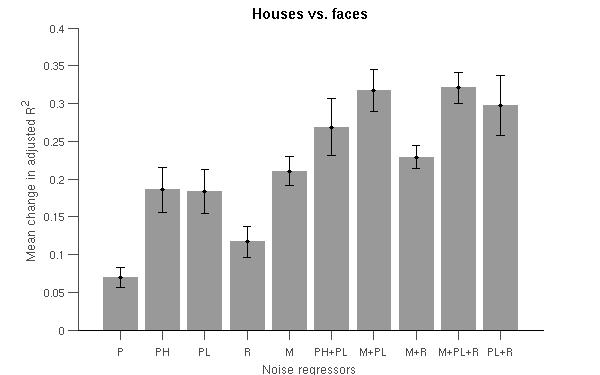
Regressors' legend: P - Pulse simple (filtered & downsampled to TR) PH - Pulse high frequency components (4 covariates) PL - Pulse: low frequency components (2 covariates) R - Respiratory simple (filtered & downsampled to TR) M - Movement (6 covariates)
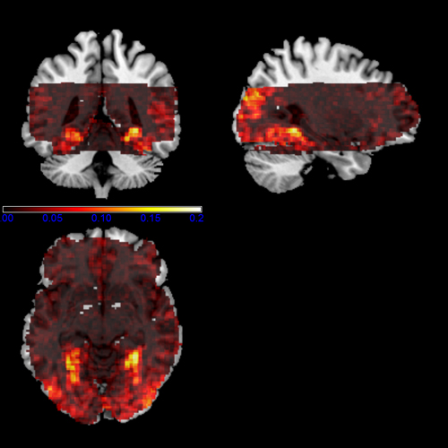
Map of voxels's change in R2 when GLM included PL and R regressors.
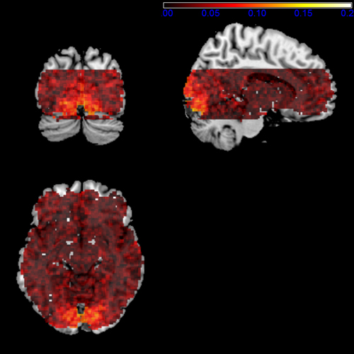
Changes in R2 distribution in the 'Houses vs. Faces' analysis
