Maxfilter Diagnostics
The output of maxfilter can be written to a text file (e.g. using the "tee" command in unix). For example, if you use movement compensation (-movecomp), this file will contain movement and HPI-fit parameters for each time step (usually every 200ms). We recommend you look at this output carefully, since it may help detect fundamental problems with HPI positioning, or whether your participant moved during a session. A possible Matlab script for reading the maxfilter output is shown below, together with a shorter script that reads the output and displays it in separate figures for each input file.
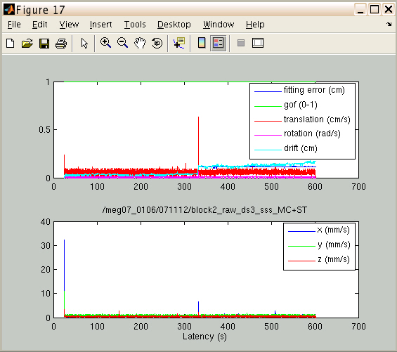
There is an example of the output below.
This script reads and displays info from maxfilter output file (if -movecomp was used):
% uses check_movecomp to read and display maxfilter -movecomp output
% Files with maxfilter outputs, e.g. for different subjects and conditions
movecompfiles = {'outputfile1.log', ...
                 'outputfile2.log', ...
                 'outputfile3.log');
nr_files = length(movecompfiles);

for ff = 1:nr_files,
    fprintf(1, 'Processing %s\n', movecompfiles{ff});
    [mv_fig, linet, linee, lineg, linev, liner, lined] = check_movecomp(movecompfiles{ff}); % read info from log-file
    [a,b,c,d] = fileparts( movecompfiles{ff} );
    tittxt = [a(end-17:end) '/' b]; % just one way to keep the figure title short
    figure( mv_fig );
    % check_movecomp only creates the figure, but without the title, so you can do this separately
    ht = title(tittxt); set(ht, 'interpreter', 'none'); % add title to figure
end;
The previous script uses the following Matlab function (also in /imaging/olaf/MEG/maxfilter):
function [mv_fig, linet, linee, lineg, linev, liner, lined] = check_movecomp(mvcomp_file);
% read and plot maxfilter output from log-file
% [mv_fig, linet, linee, lineg, linev, liner, lined] = check_movecomp(mvcomp_file);
colours = {'b', 'g', 'r', 'm', 'c', 'k', 'y'};
fprintf(1, 'Input file: %s.\n', mvcomp_file);
fid_in = fopen(mvcomp_file);    % open movecomp log-file
now_line = fgetl(fid_in);
cc = 0;
fprintf(1, 'Reading line ');
while feof(fid_in) == 0,
    if ~isempty(deblank(now_line)),
        cc = cc + 1;
        alllines{cc} = now_line;
        if ~mod(cc,100), fprintf(1, '%d ', cc); end;
        if ~mod(cc,1000), fprintf(1, '\n', cc); end;
    end;
    now_line = fgetl(fid_in);
end;    % while...
nr_lines = cc;
fprintf(1, '\n%d lines read\n', nr_lines);
HPIline = 'Hpi fit OK, movements [mm/s]';
lenH = length(HPIline);
Tline = '#t =';
lenT = length(Tline);
c_fit = 0;
t_fit = 0;
for cc = 1:nr_lines,
    thisline = alllines{cc};
    n = length(thisline);

    if n>=lenH && strcmp(thisline(1:lenH),HPIline),
        c_fit = c_fit+1;
        [tmp, restof] = strtok(thisline, '=');
        [tmp, restof] = strtok(restof(2:end), '/');
        cnt=0;
        while ~isempty(deblank(restof)),
            if length(find(findstr(tmp, '-')))==0,
                cnt=cnt+1;
                xyz(cnt,c_fit) = str2num(tmp);
            end;
            [tmp, restof] = strtok(restof(2:end), '/');
        end;
    end;

    if n>=lenT && strcmp(thisline(1:lenT),Tline),
        t_fit = t_fit+1;

        [tmp, restof] = strtok(thisline, 't');
        [tmp, restof] = strtok(restof, '=');
        [tmp, restof] = strtok(restof, ',');
        linet(t_fit) = str2num( tmp(2:end) );

        [tmp, restof] = strtok(thisline, 'e');
        [tmp, restof] = strtok(restof, '=');
        [tmp, restof] = strtok(restof);
        [tmp, restof] = strtok(restof);
        linee(t_fit) = str2num( tmp(2:end) );

        [tmp, restof] = strtok(thisline, 'g');
        [tmp, restof] = strtok(restof, '=');
        [tmp, restof] = strtok(restof);
        [tmp, restof] = strtok(restof, ',');
        lineg(t_fit) = str2num( tmp(2:end) );

        [tmp, restof] = strtok(thisline, 'v');
        [tmp, restof] = strtok(restof, '=');
        [tmp, restof] = strtok(restof);
        [tmp, restof] = strtok(restof);
        linev(t_fit) = str2num( tmp(2:end) );

        [tmp, restof] = strtok(thisline, 'r');
        [tmp, restof] = strtok(restof, '=');
        [tmp, restof] = strtok(restof);
        [tmp, restof] = strtok(restof);
        liner(t_fit) = str2num( tmp(2:end) );

        [tmp, restof] = strtok(thisline, 'd');
        [tmp, restof] = strtok(restof, '=');
        [tmp, restof] = strtok(restof);
        [tmp, restof] = strtok(restof);
        lined(t_fit) = str2num( tmp(2:end) );

    end;

end;
mv_fig(1) = figure;
subplot(2,1,1);
plot(linet, linee, colours{1}, linet, lineg, colours{2}, linet, linev, colours{3}, linet, liner, colours{4}, linet, lined, colours{5});
%legend( {'#e (cm)', '#g', '#v (cm/s)', '#r (rad/s)', '#d (cm)'} );
legend( {'fitting error (cm)', 'gof (0-1)', 'translation (cm/s)', 'rotation (rad/s)', 'drift (cm)'} );
if exist('xyz', 'var') && ~isempty(xyz),
    if size(xyz,2)~=length(linet),
        linet = 1:size(xyz,2);
        fprintf(1, '\n\nHPI problems!!! %s\n\n', mvcomp_file);
    end;
    subplot(2,1,2);
    plot(linet, xyz(1,:), colours{1}, linet, xyz(2,:), colours{2}, linet, xyz(3,:), colours{3});
    legend( {'x (mm/s)', 'y (mm/s)', 'z (mm/s)'} );
else,
    fprintf(1, '\n\nHPI problems!!! %s\n\n', mvcomp_file);
end;
Here's an example of how the output might look like:

The upper panel is the more important one. The green line (goodness-of-fit, "gof") indicates how well the HPI coils could be detected, and should always be 1 (without accurate localisation of these coils, the rest would be meaningless). Translation (red), rotation (pink) and drift (light blue) indicate whether the subject moved their head. These values should be as low as possible, ideally below 0.3. As this example shows, this recording went rather well, with some sudden movements occurring at the beginning and around the middle of the scan.
